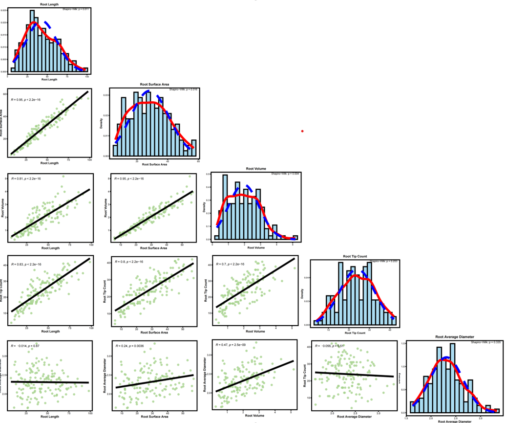
做GWAS表型很多，不可能一个一个作图，所以对表型数据进行批量分析，利用AI写了一个R代码

用的表型数据形式如下：

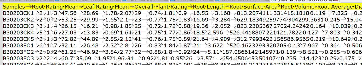
第一列为样本为，之后每一列是一个表型，中间用制表符分隔开。

一、直方图分析

# 1. 加载所需包 ----------------------------------------------------------------
if (!require("tidyverse")) install.packages("tidyverse")
if (!require("ggpubr")) install.packages("ggpubr")
library(tidyverse)
library(ggpubr)

# 2. 设置工作路径并读取数据 ----------------------------------------------------
setwd("D:/1、博士期间/9、博士-实验以及项目/12、根腐病GWAS/基因型填补")
df_raw <- read.delim("表型作直方图文件20260318.txt", 
                     sep = "\t", 
                     row.names = 1,
                     check.names = FALSE,
                     stringsAsFactors = FALSE)

# 获取所有性状名称
all_traits <- colnames(df_raw)
cat("共有", length(all_traits), "个性状：\n")
print(all_traits)

# 创建输出文件夹
output_dir <- "histograms"
if (!dir.exists(output_dir)) dir.create(output_dir)

# 3. 定义绘图函数（单个性状的直方图 + 正态曲线 + Shapiro-Wilk p值）-----------
plot_histogram <- function(data, trait, out_dir) {
  # 提取性状数据并删除缺失值
  vec <- data[[trait]]
  vec <- vec[!is.na(vec)]
  n <- length(vec)
  
  if (n < 3) {
    cat("跳过", trait, "：样本数不足", n, "\n")
    return(NULL)
  }
  
  # 计算Shapiro-Wilk正态性检验p值（当样本量在3~5000之间）
  sw_test <- shapiro.test(vec)
  p_value <- sw_test$p.value
  p_label <- ifelse(p_value < 0.001, "p < 0.001", 
                    paste("p =", formatC(p_value, format = "f", digits = 3)))
  
  # 计算均值和标准差用于正态曲线
  mean_val <- mean(vec)
  sd_val <- sd(vec)
  
  # 生成安全文件名
  safe_name <- gsub("[^A-Za-z0-9]", "_", trait)
  filename <- file.path(out_dir, paste0(safe_name, "_histogram.pdf"))
  
  # 绘制直方图 + 密度曲线 + 理论正态曲线
  p <- ggplot(data.frame(x = vec), aes(x = x)) +
    geom_histogram(aes(y = after_stat(density)), 
                   bins = 20, fill = "skyblue", color = "black", alpha = 0.7) +
    geom_density(color = "red", linewidth = 1, linetype = "solid") +
    stat_function(fun = dnorm, args = list(mean = mean_val, sd = sd_val),
                  color = "blue", linewidth = 1, linetype = "dashed") +
    annotate("text", x = Inf, y = Inf, 
             label = paste0("Shapiro-Wilk: ", p_label), 
             hjust = 1.1, vjust = 1.5, size = 4, color = "black") +
    labs(title = trait, x = trait, y = "Density") +
    theme_bw() +
    theme(
      plot.title = element_text(hjust = 0.5, face = "bold", size = 14),
      axis.text = element_text(face = "bold", size = 10),
      axis.title = element_text(face = "bold", size = 12),
      panel.border = element_rect(color = "black", linewidth = 0.8, fill = NA),
      panel.grid.major = element_blank(),
      panel.grid.minor = element_blank()
    )
  
  # 保存
  ggsave(filename = filename, plot = p, width = 6, height = 5)
  cat("已保存:", filename, "样本数:", n, "\n")
}

# 4. 批量生成所有性状的直方图 -------------------------------------------------
for (trait in all_traits) {
  plot_histogram(df_raw, trait, output_dir)
}

cat("全部完成！共生成", length(all_traits), "个PDF文件，保存在", output_dir, "文件夹中。\n")

二、相关性分析

# 1. 安装并加载所需包 --------------------------------------------------------
if (!require("tidyverse")) install.packages("tidyverse")
if (!require("ggpubr")) install.packages("ggpubr")
library(tidyverse)
library(ggpubr)

# 2. 设置工作路径并读取数据 ----------------------------------------------------
setwd("D:/1、博士期间/9、博士-实验以及项目/12、根腐病GWAS/基因型填补")
df_raw <- read.delim("表型作直方图文件20260318.txt", 
                     sep = "\t", 
                     row.names = 1,
                     check.names = FALSE,
                     stringsAsFactors = FALSE)

# 查看列名
all_traits <- colnames(df_raw)
cat("共有", length(all_traits), "个性状：\n")
print(all_traits)

# 创建输出文件夹
output_dir <- "pairwise_correlations"
if (!dir.exists(output_dir)) dir.create(output_dir)

# 3. 定义绘图函数（使用ggplot2 + .data[[ ]] 避免特殊字符问题）-----------------
plot_pair <- function(data, trait1, trait2, out_dir) {
  # 提取数据并删除缺失值
  df_plot <- data[, c(trait1, trait2)]
  df_plot <- df_plot[complete.cases(df_plot), ]
  n <- nrow(df_plot)
  
  # 如果样本数太少（如<3），跳过绘图
  if (n < 3) {
    cat("跳过", trait1, "vs", trait2, "：样本数不足", n, "\n")
    return(NULL)
  }
  
  # 生成安全文件名（替换空格和特殊字符）
  safe_name1 <- gsub("[^A-Za-z0-9]", "_", trait1)
  safe_name2 <- gsub("[^A-Za-z0-9]", "_", trait2)
  filename <- file.path(out_dir, paste0(safe_name1, "_vs_", safe_name2, ".pdf"))
  
  # 绘制图形
  p <- ggplot(df_plot, aes(x = .data[[trait1]], y = .data[[trait2]])) +
    geom_point(color = "#a6d38d", size = 3, alpha = 0.7) +
    geom_smooth(method = "lm", se = FALSE, color = "black", linetype = "solid", linewidth = 0.8) +
    stat_cor(method = "pearson", 
             label.x.npc = "left",
             label.y.npc = "top",
             size = 5,
             digits = 2) +
    labs(x = trait1, y = trait2) +
    theme_bw() +
    theme(
      panel.border = element_rect(color = "black", linewidth = 0.8, fill = NA),
      axis.text = element_text(face = "bold", size = 12),
      axis.title = element_text(face = "bold", size = 14),
      panel.grid.major = element_blank(),
      panel.grid.minor = element_blank()
    )
  
  # 保存
  ggsave(filename = filename, plot = p, width = 6, height = 5)
  cat("已保存:", filename, "样本数:", n, "\n")
}

# 4. 生成所有两两组合并绘图 ---------------------------------------------------
trait_combinations <- combn(all_traits, 2, simplify = FALSE)

for (i in seq_along(trait_combinations)) {
  trait_pair <- trait_combinations[[i]]
  trait1 <- trait_pair[1]
  trait2 <- trait_pair[2]
  plot_pair(df_raw, trait1, trait2, output_dir)
}

cat("全部完成！共生成", length(trait_combinations), "个PDF文件，保存在", output_dir, "文件夹中。\n")

示意图片: